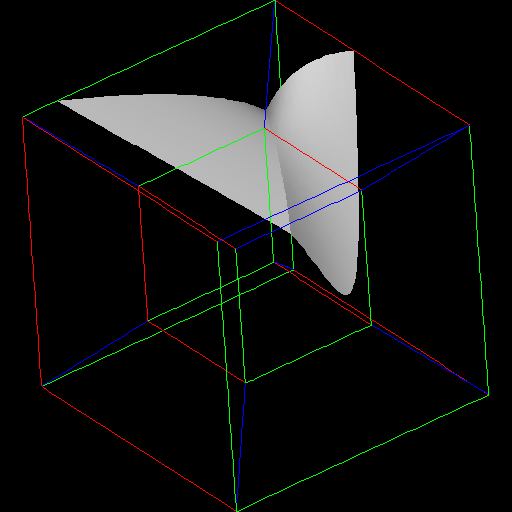
Visualizing 4D Hypercube Data By Mapping Onto a 3D Tesseract
Alan B. Scrivener
(c) 1996
as submitted for presentation as a Research Paper at the ACM/SIGGRAPH '96
Conference held August 4-9, 1996 in New Orleans, Louisiana
Keywords:
visualization, four dimensional, hypercube, tesseract, isosurface
ABSTRACT
More and more data sources are giving us higher-dimensional data,
and techniques are needed to probe and display patterns in this data.
This paper demonstrates the technique of mapping 4-D data onto a
3-D tesseract (4-D hypercube projected into 3-D space) and using
isosurfaces to visualize data in the resulting irregular volumes.
THE NEED TO VISUALIZE 4D DATA
The last decade has seen explosive growth of the use of three dimensional
computer graphics for the display of quantitative information. The three
dimensions of the computer generated image have been used to represent the
familiar three spatial dimensions of geometric objects as well as more esoteric
parameter dimensions in higher order state spaces. Typically only three
dependent
variables are represented at one time, and for many uses this is
sufficient. But there is some data which is by nature four-dimensional and
defies efforts to
reduce it. Meanwhile, driven by price reductions, many
visualization techniques are now migrating from scientific and engineering uses
to business and commercial applications. The new field of data mining offers a
new source of high-dimensional data from corporate databases, for example
historical consumer purchasing information. In the visual search for correlations
in such data tools for probing four dimensions will be increasingly useful.
ANATOMY OF A HYPERCUBE
Let's say that some data 4-D exists which needs to be visualized. It is in a di
sk
file of numbers, 32x32x32x32 of them, which are meant to be read into a
four-dimensional array in the computer's memory. So far this is trivial to do. Bu
But
assigning geometric meaning to that 4-D data is challenging. The data is in
a
hypercube, the 4-D generalization of a 3-D cube. Although a hypercube cannot
be seen by humans, we can learn much about it by analysis. Consider the
following evolution.
Moving a point a unit length in any direction yields a line segment, which is
bounded by two points. Moving that line segment a unit length in a
perpendicular direction yields a square, which is bounded by four line
segments and four points. Moving that square in a perpendicular direction
yields a cube, bounded by six squares, twelve line segments and eight points.
The formula for these numbers can be generalized. Move a primitive of
dimension N
in a perpendicular direction to its components and you will get:
- for primitives of dimension M, two times the number you started with plus the
number of primitives you had of dimension M-1
In the case where M=N+1, you get one, since the number you started with was
zero. In the case where M=0, points, you get twice the number of points you
started with, since there are no primitives of dimension less than zero. In all
other cases the values can be found recursively.
So continuing with the cube, you move it in a perpendicular direction
and you
get one hypercube, eight cubes, twenty-four squares, thirty-two line segments,
and sixteen points. This information is summarized in the following table:
component numbers of primitives in dimensional primitives
| primitive |
points |
lines segments |
squares |
cubes |
hypercubes |
| point |
1 |
0 |
0 |
0 |
0 |
| line segment |
2 |
1 |
0 |
0 |
0 |
| square |
4 |
4 |
1 |
0 |
0 |
| cube |
8 |
12 |
6 |
1 |
0 |
| hypercube |
16 |
32 |
24 |
8 |
1 |
Most values are given by two times the number above plus the number to the
upper left. Thus the entries in this table can be determined by simple arithmetic.
Figuring out what it means is tougher.
ANALOGIES TO LOWER DIMENSIONS
A way to "sneak up" on a four dimensional visualization is to use analogies from
lower dimensions. Inhabitants of "flatland" would have trouble imagining a
cube. If you told them it was bounded by six squares, twelve line segments and
eight points, they would say there is no such figure, and besides, a square can't
bound anything, since is fills (2D)
space. If you said you generated a cube by
moving a square in a perpendicular
direction, they would tell you there is no
such direction. You could show them
an unfolded cube (Figure 1), and tell them
that these six squares can be folded up into a cube, with each square rotating
about a line segment it borders on.
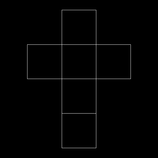 They would say that there is no way to
rotate about a line segment. You could show them projections of a cube, both
without perspective (Figure 2) and with it (Figures 3a and 3b).
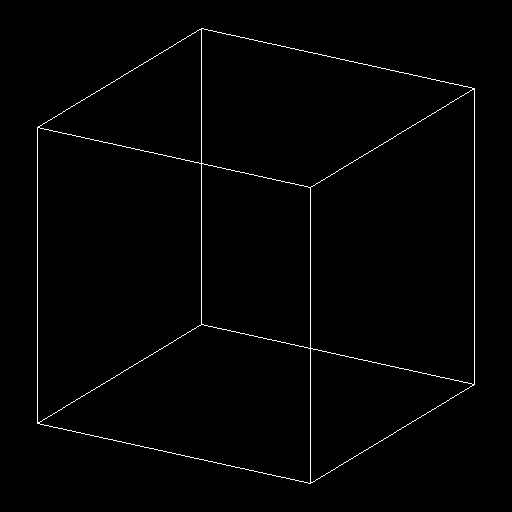
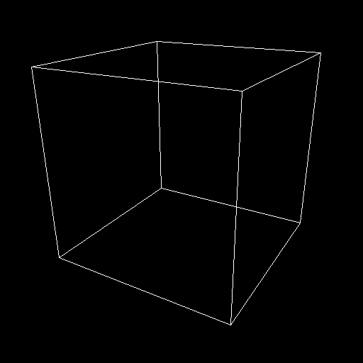
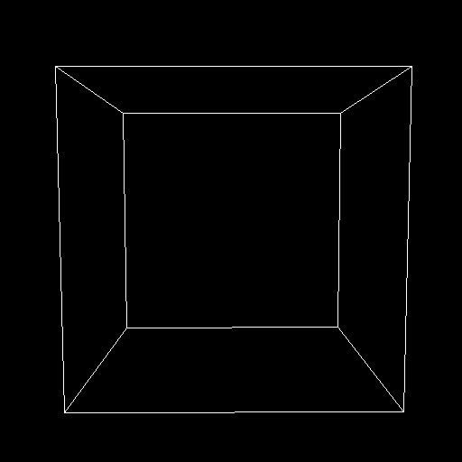 These last two
might confuse them, and lead them to
ask why the one square is sometimes
inside the other and sometimes isn't. You
would have to tell them that the one
square is never inside the other, because
this is only a projection. You would
probably also have to remind them that all the oddly shaped quadrilaterals in
the pictures were in fact true squares, with right angles and equal sides. The
Flatlanders would probably be confused by this.
Now what if hyperbeings came to us to tell us about the hypercube? If they told
us it was bounded by eight cubes, twenty-four squares, thirty-two line
segments
and sixteen points, we would say there is no such figure, and besides, a cube
can't bound anything, since is fills (3D) space. If they said you generated a
hypercube by moving a cube in a perpendicular direction, they would tell you
there is no such direction. They could show us an unfolded hypercube (Figure
4), and tell us that these eight cubes can be folded up into a cube, with each
cube rotating about a square it borders on.
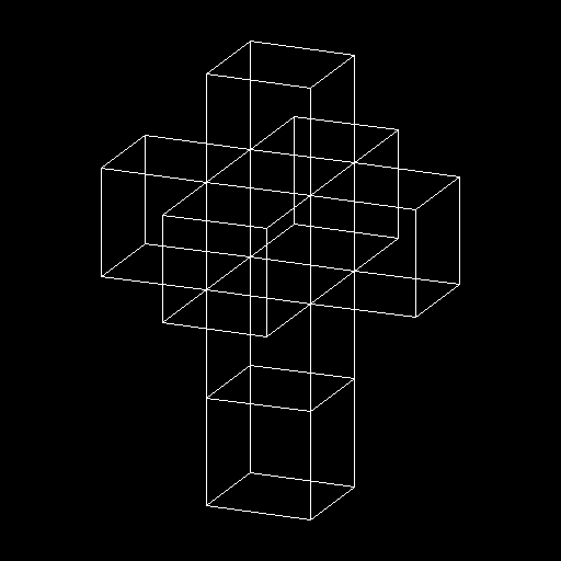 We would say that there is no way
to rotate about a square. They could show us projections of a hypercube, both
without perspective (Figure 5) and with it (Figure 6a).
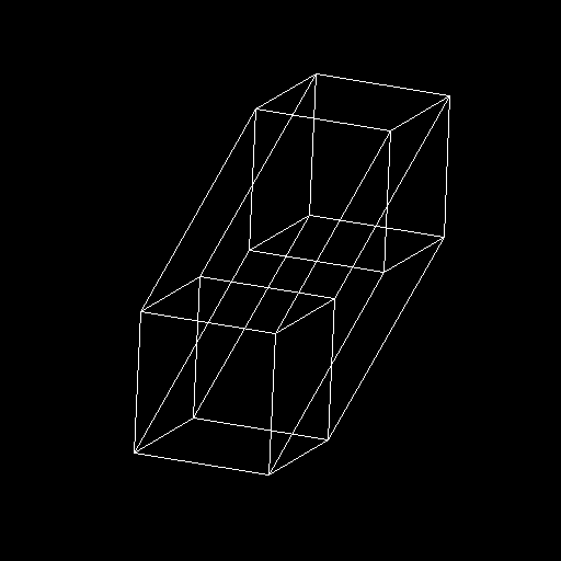
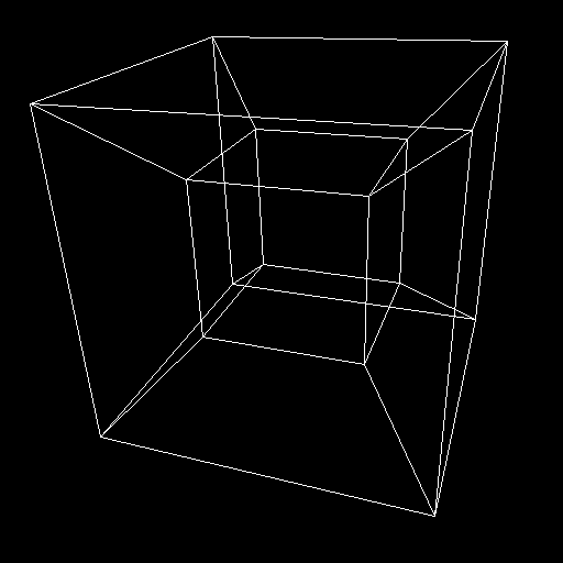 These last two
might confuse us, and lead us to ask why the one cube is sometimes inside the
other and sometimes isn't. They would tell us that the one cube is never inside
the other, because this is only a projection. They would probably also have to
remind us that all the oddly shaped hexahedrons in the pictures were
in fact
true cubes, with right angles and square faces. We would probably be
confused by this.
MAPPING TO A TESSERACT
The tesseract (Figure 6b) gives us
what this author believes is the best avenue
to visualizing 4-D data. The eight bounding cubes can be identified: the large
outer cube, the smaller inner cube, and the six trapezoids that connect them.
The relationships between the cubes are visible as well. Each is surrounded by
six others, and shares a square
face with each. Furthermore, because of
perspective, parts of the figure that
are farther away in the 4th dimension (let's
call it the "w" direction) are smaller. It is as if moving in the +w direction makes
things colder, and they shrink uniformly.
To name the parts of the tesseract, let us assume it is oriented on a compass
rose on the ground, and we are south of it, looking north. The
(trapezoid) cube
closest will be the South Cube, and the one farthest away the
North Cube. The
other four trapezoids then become the East, West, Top and Bottom Cubes. The
outer cube, which is closest in w, let's call the Hither Cube, and call the smaller
inner cube, which is farthest in w, the Yon Cube. Let us
assume that all
coordinate values range from zero to one as well. To number the points in the
figure, construct a binary number for each point where the w value is the eight's
place, the x value the four's place, the y value the two's place, and the z value
the one's place. Two opposite diagonals are 0000 = 0 and
1111 = 15.
Consider the West Cube, which is on our left. This cube represents
a 3-D slice
of the 4-D hypercube where x=0. Since x is held constant, in this
trapezoid the
x direction is appropriated for showing w instead. Likewise the
East Cube also
uses the x direction for w, since it is a slice where x=1. Th
e Top and Bottom
Cubes show slices for y=1 and y=0 respectively, and use the y
axis to show w.
And of course the Front and Back Cubes show slices at z=0 and
z=1
respectively and use the z axis to show w.
Armed with the above informati
on, it becomes possible to map 4-D data onto
the 3-D tesseract. remembering ou
r 32x32x32x32 array in memory, here is
what we do with it. Consider the front
bottom leftmost point of the Left Cube. Its
4-D coordinates are {0, 0, 0, 0},
and so its number is 0000 = 0. Its data value is
simply the value at [0][0][0
][0] in the array, while its 3-D coordinates are {0.0, 0.0,
0.0}. Now conside
r the front bottom rightmost point of the Left Cube. Its 4-D
coordinates are {
0, 0, 0, 1}, and so its number is 0001 = 1. Its data value is the
value at [0
][0][0][31] in the array, while its 3-D coordinates are {0.25, 0.25, 0.25}.
A
ny points on a line between these two can have both their coordinate and data
v
alues determined directly by interpolation between 0000 and 0001. All other
p
oints can be calculated by further interpolation.
Once the 4-D data is mapped i
nto the 3-D tesseract shape, isosurfaces can be
calculated inside each trapezoi
d and cube if desired. These will represent
surfaces of constant value in a cu
be where one 4-D coordinate is at its minimum
or maximum. Up to four such surf
aces can be combined before -- in general --
surfaces will begin to obscure eac
h other.
TWO EXAMPLES
First, we look at a light cone form Einstein's Special
Theory of Relativity. This is
a 4-D hypercone for all values in space-time for
which:
sqrt(x^2 + y^2 + z^2 - t^2) = 0
This structure has particular phy
sical significance because, relative to an
observer at the origin, all 4-D spac
e-time points on the hypercone are "light-like"
(able to transfer information to or from the observer only if moving at velocity c),
while all 4-D points inside the positive and negative ends of the hypercone are
"time-like" (able to transfer information to or from the observer at velocities less
than c) and all 4-D points outside the hypercone are "space-like" (unable to
communicate with the observer).
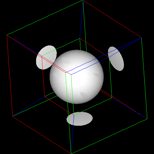
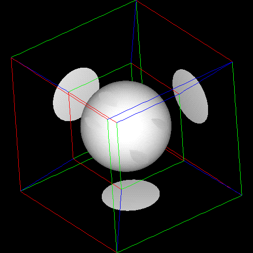
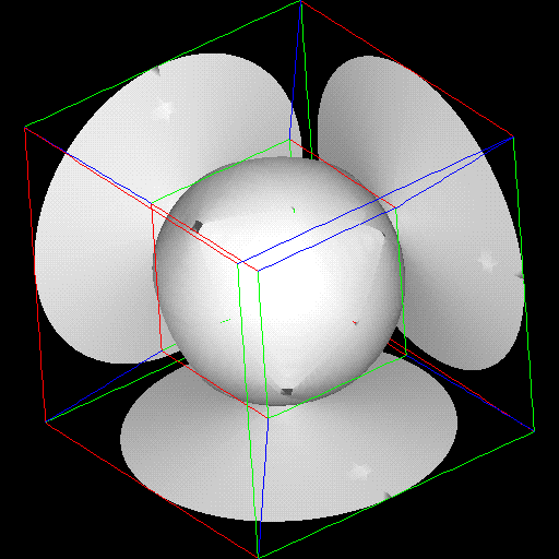
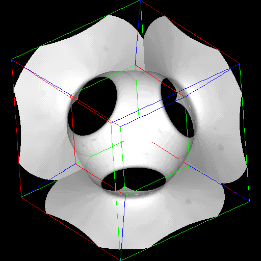
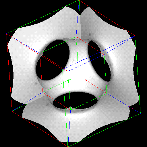
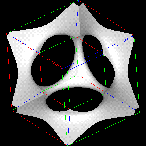
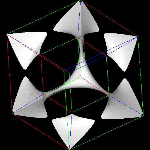
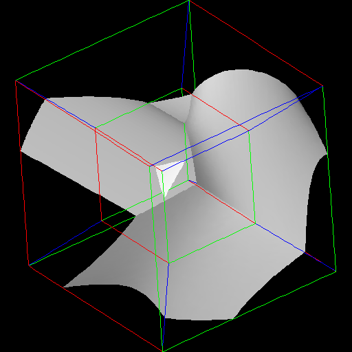
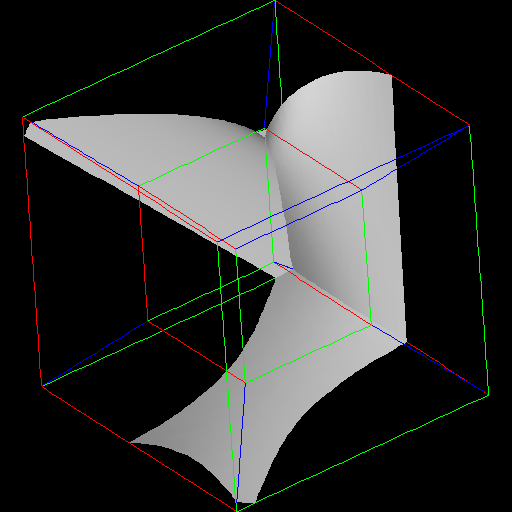
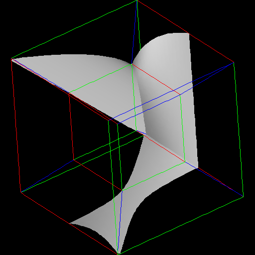
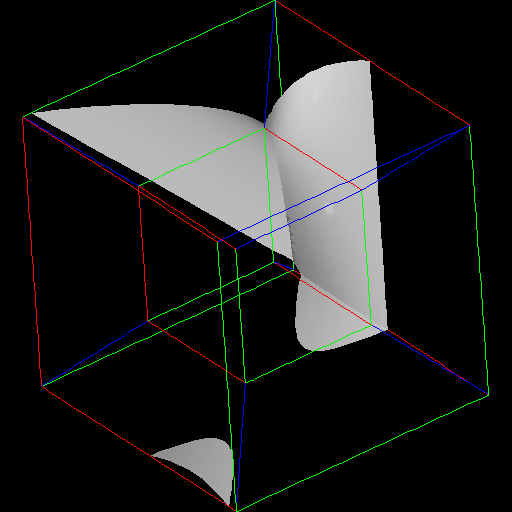
By filling the 4-D array with the values given by the above equation and then
generating the four cubes where each variable (x, y, z and w) is in turn held at
zero -- in other words the Yon, Left, Back and Bottom Cubes -- I was able to
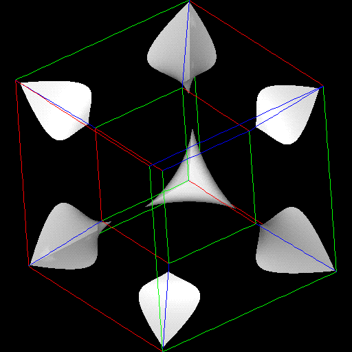
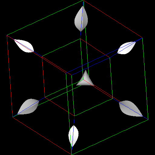
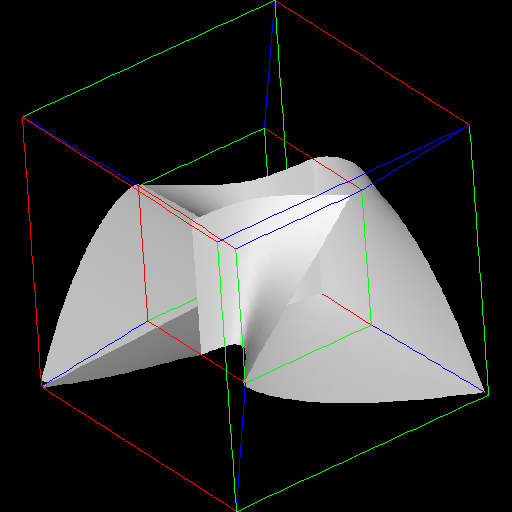
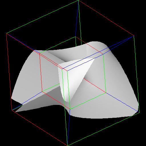
produce the visualization shown in Figures 7a-k. Only the value of the
isosurface constant is changing in the pictures. The 3-D spherical symmetry of
the shape is readily aparrent as a spacial duplication of pattern, looking almost
like flowering shapes.


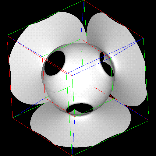
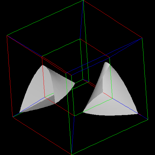
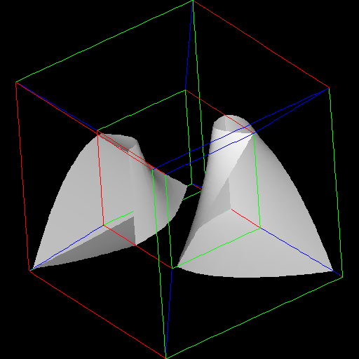
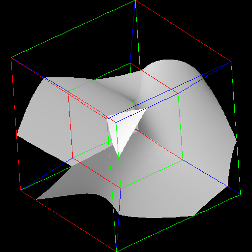
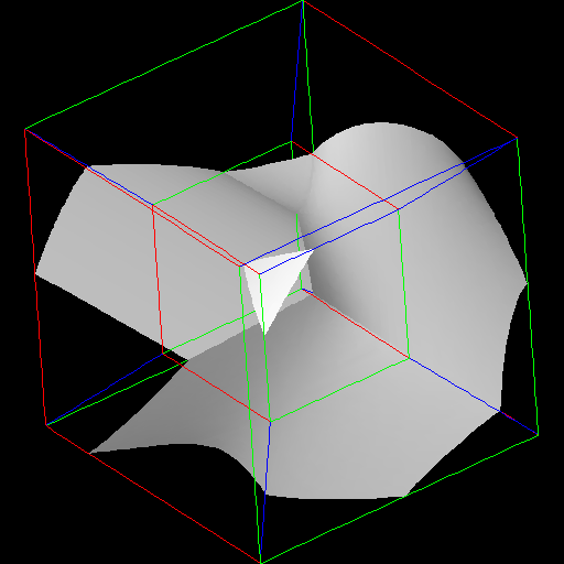
The second example is a 4-D quadratic surface, given by AX^2 + BX + C = 0.
By assigning values of w, x, y and z to A, B, C and X, and ranging from -1 to 1, I
generated 4-D than was then mapped to the 3-D tesseract in the same way.
The results, isosurfaced with constants ranging from -2 to 2 in the pictures
(Figures 8a-k), show 3-D slices of 4-D surfaces. Such surfaces can often
generated in decision analysis, as surfaces of constant utility, but usually are
not because of the difficulty of displaying them. Not that where the surface
seems to crease, there is in fact a 4-D fold, analogous to the crease in an
unfolded cube.


FUTURE WORK
In the near future this technique will be applied to business data, in search of
previously undiscovered demographic trends.
REFERENCES
1.  Robert A. Heinlein "And He Built a Crooked House" published in
        Astounding Science Fiction Magazine  1940
2.  George Gamov One Two Three... Infinity   Bantam Books 1947
3.  Thomas F. Banchoff  Beyond the Third Dimension  -- Geometry, Computer
        Graphics and Higher Dimensions  Scientific American Library 1990
 We would say that there is no way
to rotate about a square. They could show us projections of a hypercube, both
without perspective (Figure 5) and with it (Figure 6a).

 These last two
might confuse us, and lead us to ask why the one cube is sometimes inside the
other and sometimes isn't. They would tell us that the one cube is never inside
the other, because this is only a projection. They would probably also have to
remind us that all the oddly shaped hexahedrons in the pictures were
in fact
true cubes, with right angles and square faces. We would probably be
confused by this.
 They would say that there is no way to
rotate about a line segment. You could show them projections of a cube, both
without perspective (Figure 2) and with it (Figures 3a and 3b).


 These last two
might confuse them, and lead them to
ask why the one square is sometimes
inside the other and sometimes isn't. You
would have to tell them that the one
square is never inside the other, because
this is only a projection. You would
probably also have to remind them that all the oddly shaped quadrilaterals in
the pictures were in fact true squares, with right angles and equal sides. The
Flatlanders would probably be confused by this.
